Oil production models with normal rate curves
Hubbert fitted the rate of U.S.A. oil production with logistic curves.
Deffeyes says that the normal curve gives a better fit. As far as I know,
there has previously been no theoretical justification of these fittings.
In my paper
Oil production models with normal rate curves
conditions ensuring approximately normal rate of production
curves are established. It has been accepted to appear in the journal
Probability in the Engineering and Informational Sciences.
Here is the abstract of the paper:
The normal curve has
been used to fit the rate of both world and U.S.A. oil
production. In this paper we give the first theoretical basis for these curve fittings. It is well known that oil field sizes can be modelled by independent samples from a lognormal distribution. We show that when field sizes are lognormally distributed, and the starting time of the production of a field is approximately a linear function of the logarithm of its size, and production of a field occurs within a small enough time interval, then the resulting total rate of production is close to being a normal curve.
We call the total rate of production the sum of the rates of production of
the fields constituting a given area.
The main idea is that the rates of production of individual fields does
not matter much in obtaining an approximately
normal total rate of production curve. What matters,
assuming the time it takes
to produce individual fields is not too long,
is the distribution of field sizes and the location in time of
their production.
Next, I will explain what is meant in the abstract. After that, I will make
some remarks about the model in the paper.
What is meant by a lognormal distribution? A normal distribution is the
familiar bell-shaped curve.
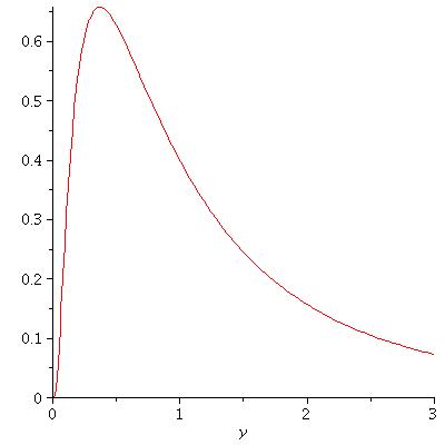
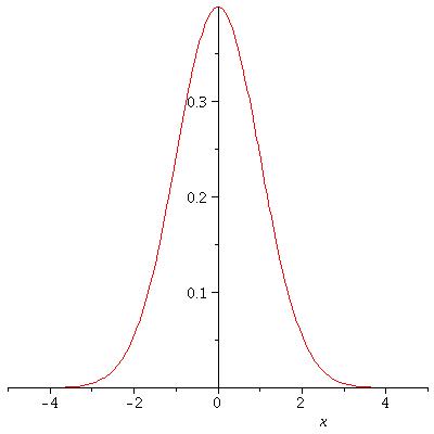 A lognormal distribution obtained by a simple transformation of the normal
distribution: if X is a normally distributed random variable,
then eX is lognormally
distributed. Here is the lognormal distribution associated with the normal
distribution above.
A lognormal distribution obtained by a simple transformation of the normal
distribution: if X is a normally distributed random variable,
then eX is lognormally
distributed. Here is the lognormal distribution associated with the normal
distribution above.
 Lognormal distributions have
been used to model the distribution of the
oil field sizes in a given area.
Moreover, the lognormal distribution
is fundamental to the Black-Scholes
model of the stock market used in the analysis of derivatives.
(Here we are
using it for something more sensible.)
Lognormal distributions have
been used to model the distribution of the
oil field sizes in a given area.
Moreover, the lognormal distribution
is fundamental to the Black-Scholes
model of the stock market used in the analysis of derivatives.
(Here we are
using it for something more sensible.)
We will suppose that oil field sizes are given by independent samples from
a lognormal distribution.
Next we suppose that the production of oil from
field of size x occurs approximately
at time -a log(x) + b, where a>0 and b are constants.
More specifically, we suppose that all the oil produced from a field of size
x occurs in the time interval ranging from
-a log(x) + b -L to -a log(x) + b + L, where L>0 is
a constant.
Under these assumptions, the rate of oil production converges to
a curve which is close to being
normal. The "converging" bit means that
the total rate of production of the first n fields
divided by the total amount of oil ever produced by the first n fields
tends to a limit curve as n tends to infinity.
What does "close to normal" mean? Let Fn(t)
be the amount of oil produced by the first n fields up to time t, divided by the
total amount of oil ever produced by the first n fields.
Suppose that the lognormal distribution describing the field sizes
is obtained from a normal distribution
with standard deviation s.
Let F(t) be the
function you would have corresponding to Fn(t)
if the rate of production was exactly normal.
It turns out that
the normal distribution corresponding to
F(t) has standard deviation roughly equal to S = as.
Let
Dn=max|Fn(t)-F(t)|,
where the maximum is taken over all time points t.
Then, when n is large enough,
Dn < L/ S.
Thus, when L/S is small, the rate of production is close
to being normal in the sense that Dn is small for n large enough.
Note that L can be large and Fn(t) still be close to normal,
as long as L/S is small.
Here are some concluding comments on the model.
- The model could be taken as applying only to fields below a certain
threshold size.
For example, the largest field
in the U.S.A. is Prudhoe Bay, which started production
later than one would expect
from its size as a consequence
of its location in the arctic. Prudhoe Bay skews the total rate of production
curve of the U.S.A. to the right,
though not enough to move the peak total rate of production away from 1970.
On the other hand, if a few smaller fields were produced earlier than
one would expect from their sizes, they would not skew the total rate
of production curve by much.
- The condition that
oil produced from a field of size
x occurs in the time interval -a log(x) + b -L to -a log(x) + b + L
probably does not need to hold precisely
for the approximation to hold. What is
intuitively important is that
production is concentrated around -a log(x) + b.
- It would be most interesting to have empirical evidence as to whether this
model describes actual oil production in some area or areas.
This should hold when
the production of fields of size x is centred about
f(x)=-a log(x) + b for some constants a>0 and b.
If such evidence exists,
then it would be desirable to find some explanation for
the appearance of the function f(x).
- The total rate of production curve is
approximately normal for U.S.A. and world oil production.
For many other areas, such as the North Sea, it is not.
This could be because the larger areas
have a wider range of field sizes and because their total rate
of production curves have greater width (which in the model is roughly equal
to S)
compared to the time intervals
individual fields are in production (which in the model is represented by L).
- The function -a log(x) +b
implies that the smallest
fields will be produced
indefinitely far into the future; any reasonable model producing a bell shaped
curve would have this feature.
This is probably an unrealistic
assumption.
Could this be part of the reason that the current rate of oil
production in the U.S.A. is higher than was predicted by Hubbert?
Another reason could be delayed production from large fields such as Prudhoe Bay.
- We have investigated lognormally distributed field sizes together with
normal total production curves for the reason that
the analysis seemed natural and elegant.
Other combinations of field size distributions and classes of total
production curves could also be studied, for example with field size
determined by independent samples from a Pareto distribution and lognormal
rate of production curves.
You can get in touch with me at D.S.Stark@maths.qmul.ac.uk